

Bookmark this if you are trying to maximise $ spent per unit of intelligence while pre-training
TLDR :-
- choose a size of the ablation model that meaningful produces signal. If your long run model size is around 30B then abalations on 500M-3B make sense.
- run cheap deterministic filters before expensive learned ones to filter data to train the ablation models above
- compare every data intervention with an equal-compute baseline and
- inspect both full-data-mixture and held-out regressions before scaling.
Early in my career, I built a lead-scoring model and learned a hard lesson of data quality and calibration of classification models. The value of doing the painful, grunt-like EDA step so i could surface the signal or at least throw away the noise. Improving data quality by manually writing pandas, was cumbersome but rewarding. That frame's this article's question:
when AI researchers are compute bound, how much capability can better data curation buy per token?
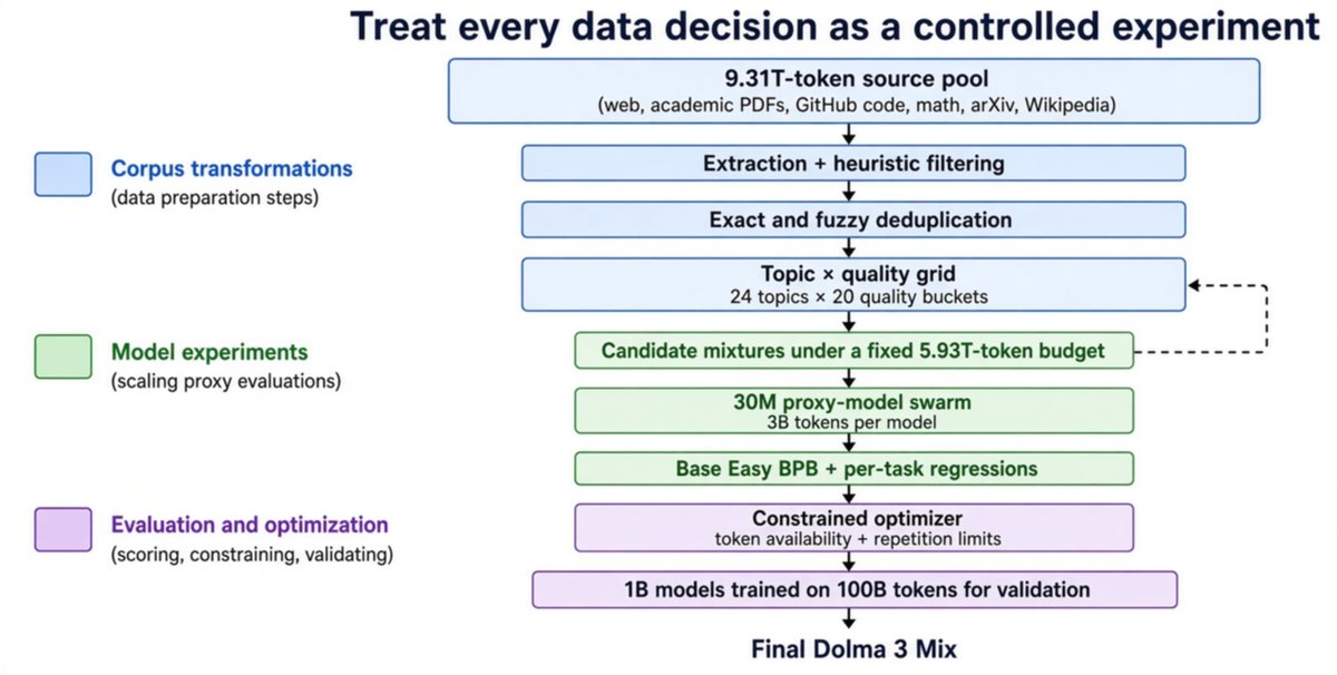
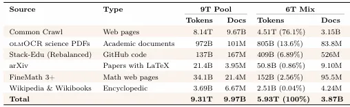
OLMo 3 tech report is an especially useful case study because @allen_ai is one of the very few AI labs to open nearly the entire research stack: training infrastructure, code, data, checkpoints, logs, and model artifacts. That transparency let me inspect not just the outcome, which is a fairly compettitive model but also the decisions connecting a 9.31T token pool to a 5.93T token training mix. This article extracts that practical decision process.
What is a good proxy metric for accuracy at small model scales?
At small model scales, accuracy scores jump around so much that a real improvement is hard to decipher from noise. Olmo addressed this by grouping evaluation into capability clusters and mapping them to eval metrics. An important metric which helps us measure a proxy for accuracy is BPB. Bits-per-byte (BPB) measures how confidently the model predicts a known correct answer, adjusted for answer length. Small models may remain near chance or zero accuracy and two models can receive the same accuracy even when one assigns subtantially more probability to the correct answer.
Mathematically,
where UTF8{y} denotes the number UTF-8 bytes in the gold answer.
Lets consider the question,
“What is the capital of Italy?”
The gold answer is “Rome” which contains four UTF-8 bytes.
Model A assigns p(“Rome”)=1/16:
Model B assigns p(“Rome”)=1/4:
Both models could still receive zero exact-match accuracy if another answer is their argmax, but BPB reveals that Model B is moving toward the correct answer.
Lower BPB is better.
- STEM/non STEM multiple-choice QA → QA BPB
- Math BPB
- Code BPB
- Code fill-in-the-middle
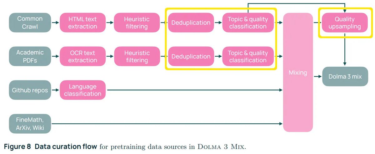
Once the evaluation signal is trustworthy, the next rule is to spend preprocessing compute from cheapest to most expensive. Commoncrawl data is very very dirty so OLMo 3 first applies lightweight heuristic filters, then removes exact duplicates with hashes before paying for fuzzy near duplicate detection and repeated-substring removal.
Cheap filtering over expensive text classification
So what does cheap filtering look like, - Heuristic filters are simple rules like too much NSFW text, blocked URLs, too little alphabetic text or too many symbols or numbers. - Compute a hash of each document’s text and keep one document per matching hash
- Fuzzy near-duplicate detection using MinHash to find likely matches then verify candidates with jaccard similarity and using suffix array based matching to find long passages repeated across otherwise different documents.
Exact matches shrink the corpus before costly similarity comparisons, while the slower language classifier runs only after cheaper commutative filters have discarded obvious noise. The goal is to remove accidental repetition first, so any later upsampling is a deliberate data-mixture decision.
Turn the corpus into 480 controllable experimental cells
OLMo 3 treats topic and quality as separate sampling decisions:
- Classify the topic using a cheap fastText classifier, distilled from WebOrganizer labels, assigns each document to one of 24 topics. Score quality separately. Another fastText classifier gives every document a learned quality score.
Documents are ranked against others in the same topic and divided into 20 five-percentile buckets.
This produces 24 × 20 = 480 controllable subsets.
The separation provides two distinct controls:
- Topic weights determine which capabilities receive training tokens.
- Quality-aware sampling determines which documents within each topic receive repetition in the pre-training datamix.
So if you've been reading until now, this is where we make use of all the artifacts we built out, Separating topic and quality creates a controllable pool, but it does not decide the final token allocation.
OLMo trained small 30M-parameter proxy models for 3B tokens on different mixtures, fitted and evaluated for each task, and searched for weights that respected token availability and repetition limits.
What should a small Lab do?
A small lab should borrow the constrained comparison, test three to five mixtures from one checkpoint with identical token counts and hyperparameters, tracking one continuous development metric, a small capability eval, and one held-out metric.
Advance ONLY clear winners.
The hidden assumption is that small-run rankings transfer, so rerun the two best candidates at a second scale before committing the final compute budget.
This looks like a 5 step procedure -->
Step 1 -> Specify the starting checkpoint or initialization policy, model architecture, tokenizer, sequence length, optimizer, learning-rate schedule, token count, and evaluation suite.
Step 2 ->Test three to five candidate mixtures or filtering policies. Do not change the model or training recipe at the same time.
Step 3 -> Every candidate must see the same number of training tokens and updates. Report repeated-token counts separately so that aggressive upsampling is visible and measurable.
Step 4 -> Track three levels of evidence = one continuous low-scale metric such as BPB; one capability-level aggregate such as Log likelihood; per-task or held-out regressions raw task accuracy.
Step 5 ->Rerun only candidates whose gains exceed run to run loss gain. Validate the top two using another seed or a second model scale{slightly bigger model to make sure the run will be stable} before spending the final compute budget.
OLMo’s 4–7× repetition constraints, classifier choices, and final mixture ratios are empirical settings, NOT universal laws.
What transfers is the experimental discipline behind them. Turn each data decision into a controlled test, When compute is expensive, every token should have to EARN its training step.